Today's Assignment: Assignment

A new R user quickly discovers that there are multiple ways to store information into an object -- the technical term for this is assignment. There's = as in:

x = c(1,2,3)

and there's <- as in:

x <- c(1,2,3)

R help on assignOps offers this explanation of the difference:

The operators <- and = assign into the environment in which they are evaluated. The operator <- can be used anywhere, whereas the operator = is only allowed at the top level (e.g., in the complete expression typed at the command prompt) or as one of the subexpressions in a braced list of expressions.

For catching subtle coding errors with =, this is a smart feature of R. When I am tired, I sometimes find myself writing a line of code that looks like this:

if(codename = "thedoctor") watch = "yes"

In this line of code, the problem is that codename = "thedoctor" isn't a logical statement. It is a statement that would assign the string "thedoctor" to an object called codename.... if the statement were allowed by R's language. Fortunately, R prevents this.

This feature of the R programming language helps me because I -- by default -- use = for assignment rather than <-. My style is not conventional, however. Popular R coding style guides (Google, 4D pie charts) suggest that users use <- option for assignment, rather than =.

Deep down, I think I use this unconventional default because I had the = versus == distinction (more generally, assignment versus logical statement) drilled into me in my first computer science class (not in R; Java). On reflection, I have three reasons to use = rather than <-. First, = is easier to type, using one keystroke and no shift keys. Second, the equals style looks cleaner to me (completely a personal preference). Third, I think assignment should take place out in the open (i.e., exactly where = is allowed). If the line of code is out in the open, both <- and = work the same.

On a final note, the <- is not without its problems for logical statements. For example, the statement

if(agediff<-2) status = "I'm older"

will cause problems and it won't let you know about these problems until you get some really strange results later on. Here's the code from an interactive R session where I show what can go wrong.

> agediff = -3
> if(agediff<-2) status = "I'm older"
> status
[1] "I'm older"
> agediff
[1] 2
> agediff = 4
> if(agediff<-2) status = "I'm older"
> status
[1] "I'm older"
> agediff
[1] 2
> status=NULL
> if(agediff<-2) status = "I'm older"
> status
[1] "I'm older"
> agediff
[1] 2

The problem is two-fold in this code. First, the if statement isn't acting as a logical statement splitting by whether "agediff< -2" Second, the value of agediff is changed because "<-" means assignment. The result is that both status and agediff have (potentially) the wrong values at the end of running the code.

As this error is a problem whether you use = or <- for assignment, it is worth knowing regardless of your style preference. Adhering to good spacing guidelines is a good way to avoid this error.

> agediff = 4
> if(agediff < -2) status = "I'm older"
> status
NULL
> agediff
[1] 4

There are some other examples in the Stack Overflow forum discussion on this topic (actually multiple threads on this), all of which are useful. It is interesting reading to be sure.

An application of aggregate() and merge()

Today, I encountered an interesting problem while processing a data set of mine. My data have observations on businesses that are repeated over time. My data set also contains information on longitude and latitude of the business location, but unfortunately, my source only started providing the longitude and latitude information in the middle of the data set. As a result, the information is missing for the first few periods for every business, but across businesses, I have latitude and longitude information for virtually all of my data set.

As long as the business hasn't shifted location, this isn't a problem. I can just substitute the lat-long information from the later periods into the earlier periods for each business. This sounds simple enough to do, but when one has a data set with 70,000 observations, an automatic process saves a lot of time and can help avoid mistakes.

Let's start by building common ground. Here is a script that you can use to simulate a data set to follow along.



Once you run this script, the data frame mydat is a balanced panel of 125 businesses observed over 25 time periods (my actual data set is an unbalanced panel and the solution I present works just as well for unbalanced as with balanced. It is just easier to simulate a balanced panel). Each observation has a business identifier (BusID), a time period identifier (per), as well as simulated data on latitude and longitude.

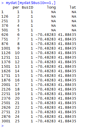
To see the problem with this data set, examine the data for the first business using the command mydat[mydat$BusID==1,]. Here's a screenshot of the output.



This problem occurs throughout the data set and we would like to just substitute the lat-long values we have for the right missing ones.

How did I solve my NA problem? I used aggregate(), a function that quickly and conveniently collapses a data frame by a factor or list of factors. With aggregate(), you can take the mean, compute the max, compute the min, sum the values or compute the standard deviation by the levels of the collapsing factor. The aggregate() function also has a na.rm option that allows us to easily ignore the NA values (useful here). In our example, we could collapse by taking the mean or computing the max or the min; the result will be the same because latitude and longitude do not vary for the same business over time.

Let's collapse by taking the mean withing each level of BusID. The result of my use of aggregate() is a data frame that upon merging with the original data frame (using merge()), fills in the missing latitude and longitude values. The following code implements this strategy to fill in the NAs in our simulated data set.



Before leaving you to have fun with aggregate() and merge(), several points are worth mentioning.

First, the aggregate() function requires that the collapsing factor(s) is (are) stored in a list. This is why the code uses list(BusID=mydat$BusID) when mydat$BusID would seem more natural. The list() part is necessary to get aggregate() to work.

Second, it is useful for merging in the second step to give the attribute in the list the same name as the variable name in the original data frame. The BusID= part of the list(BusID=mydat$BusID) command is a convenient way to prepare the resulting data frame for merging.

Third, my code uses -c(3,4) to drop the 3rd and 4th columns of the original data frame (the ones with the original lat-long data) before merging it with the collapsed latlong data frame. This is important so that the merge() command doesn't get confused about which columns to use for matching. If you leave these columns in mydat, R's merge will try to match the values in those columns as well (because they have a common name with those columns in latlong).

Finally, the data in this example are in a different order now that we merged on BusID. If this bothers you, you can use order to sort the data set by time period as in

myfinaldat=mycleandat[order(mycleandat$per),]

As this last step is purely a cosmetic change to the data set that will not affect subsequent analyses, you can leave it out.

Although this example was my solution to a rather specific problem, it illustrates how to use some useful commands. To the extent that these commands are widely applicable to other problems, I hope you find uses for these commands in related applications.

Recreational R: Simulating a Card Trick

In this post, I simulate an interesting card trick, which was described by a friend of mine named Xan. Here's Xan's description of the card trick:

• I put a deck of cards down face up on the table. Meanwhile you think of a secret number between 1 and 10 -- for exposition let's say you pick 4.
• One by one, I discard cards from the top of the deck. When we get to the 4th card -- and let's call it your special card -- you look at the number. For exposition, let's say your special card happens to be a 7. Then 7 secretly becomes your new number. Note that I don't know your special card.
• I keep flipping cards, and 7 cards later, you have a new special card and number yet again. Note that I still don't know your special card.
• This process continues -- me flipping cards at a constant rate, you secretly updating your special card and counting up to the next one -- until I decide to stop.

But I don't just stop on any card. I stop on your current special card. Which I'm not supposed to know.

The following script file is a crude first approximation to simulating this card trick for the first 150 cards. This crude strategy is simple: (1) Simulate a sequence of 150 cards, (2) Pick a starting value -- might as well do all of them at once, and (3) Implement Xan's trick on all of them (that's what the for loop does).



Here's the result of running this script three times and plotting 10 secretnum sequences: one for each starting value. Each run starts with 10 distinct secret numbers (with a default chance of 0.1 of the trick "working"), and in my three runs, every starting value of the secret number eventually converges on the same sequence of secret numbers. More on the intuition for this here.



There are a couple of things wrong with this simulation that may have stacked the deck in favor of it working. I fixed these before writing this post, but I think it is useful to see the quick and dirty solution before adding frills and realism (which is what I do now).

1. I merely simulated my 150 cards using a uniform distribution on 1 to 13 (then forcing the face cards 11, 12 and 13 to be 10s). This is equivalent to sampling with replacement, which may have different properties than sampling without replacement.
2. There are only 52 cards in a deck. How would this work with only one shuffle, but passing through the deck (almost) three times until 150 cards? This is a different problem. Maybe you wouldn't expect much improvement after one pass through the deck (because you've seen that sequence of cards before).

A clever use of the rep() command can create a "fresh" deck of cards without suit distinction (which doesn't matter for the trick). Now, how to use R to shuffle a deck of cards? The sample() command, of course. With this technique in mind, I wrote the following function to compute the probability that the trick works (that is, the probability that two independent guesses end up at the same secret number) given a number of decks and a number of passes through the entire stack of cards (for a given shuffle).



Once you define this function, we can save the probability of the trick working for 1000 different shuffles of the cards. This script does it for one deck and one pass through the deck.



Then, we can take the average probability, which feels like the probability the trick works (unconditional on the particular shuffle or guess of a secret number). In the simulations I have run, this number turns out to be around 0.74 for one deck and one pass through the deck and about 0.86 using one deck and passing through twice. There's not much improvement after the second pass through of the deck.

In case you're interested, here are the results for up to 3 decks and up to 5 passes through the set of cards. It is always better to have more decks, but two passes through two decks is about enough to virtually guarantee that the trick works.



Update: In case you are wondering, I also coded it up with a 0.01 probability of forgetting to update on any given flip of the card. Here's the table of results in this case.



It's no surprise: For forgetful people, the trick is less successful and there isn't much point in reaching for a second deck.

An Application of boot() to IV regression

Bootstrapping standard errors can be a useful technique when obtaining closed form for the standard error formula is difficult or intractable. In this post, I give an example of how to use R to create a bootstrap sampling distribution in the context of IV regression. Specifically, I use boot() to automatically augment a function of mine to resample the indices of my data set with replacement (see the code in the function below).

In my application, I present a function that uses the boot library to report bootstrap standard errors for an instrumental variables regression. My ivboot() function builds on the iv() command I wrote for the tonymisc library.*

Now, onto the ivboot() example. Start by loading the tonymisc library and some data from the library, as well as the boot library.



We can run the following R script to define the function ivboot().



When applied to data and an IV regression model, the ivboot() function creates an IV regression object that -- when tonymisc is loaded -- is compatible with mtable() output. The only difference between an ivboot()-created object and an iv() object is that the ivboot() object has standard errors that are based on the bootstrap distribution of the coefficient estimates (Statistics other than the second-stage coefficient estimates are not bootstrapped).

Here is some code to compare the bootstrap output to the analytical standard error output:



On this small sample (N=100) of simulated data, the ivboot() command took less than a minute to run on my computer (timing of may vary depending on your computer). For much larger data sets, this will be slower. If you have a larger problem or lower standards (or higher standards, your choice), you can use the boots option to ivboot() to specify the number of bootstrap samples. Currently, I have set the default to 500, but you could specify boots = 200 if you want the command to run faster (boots = 10 will make it run even faster, but I don't recommend that!).

Here is the mtable() output, which can easily be ported into LaTeX using the toLatex() command.


*This standard output from an mtable() extension to my iv() command provides quite a bit of information in a convenient format. Another nice feature of iv() is that iv()-created objects have first-stage summary information readily stored in the object for extraction and analysis.

Defaults, Lists and Classes: A Functional Post

In this post, I demonstrate a couple of useful tricks to writing functions in R. The context is a function I wrote called called samp() that allows for an easy demonstration of sampling distribution properties.



Defaults

By default, this function draws K = 500 samples of size N from a normal distribution with a mean of mu = 0 and a standard deviation of std = 1. As you can see, the syntax for specifying a default for an argument to the function is to set it equal to its default value inside the function statement. Arguments can be given no default by naming them as an argument to the function without specifying their default value.

Sensibly chosen defaults can save a lot of time for people who use your function. For example, although this samp() function has four arguments, I don't need to type samp(100, 0, 1, 500) every time I wish to take 500 samples of size N=100 from a Normal(0,1) random variable. If sampling from a Normal(0,1) is especially common, setting the defaults this way can save a lot of keystrokes.

On the other hand, using defaults instead of hard coding the Normal(0,1) choice has the distinct advantage that users get flexibility from your function giving them the option to specify arguments other than the default. The right use of defaults strikes the perfect balance between ease of use and flexibility.

Returning a List... with Names

If your function warrants the special treatment, you have probably performed several useful calculations that you would like to return. Maybe you have conducted several related hypothesis tests that you would like to reference later (report and/or use in another calculation). A great way to do this is to store the results of your function into a list.

For example, in the samp() function, I wanted to store vectors of the sample means, sample standard deviations and standard errors (500, one for each replication). For good measure, I wrote the function to store the means and standard deviations of these vectors as well as the true parameter values that went into the function.

Although it is often a good idea to store the results in a list, it is a better idea to name the elements of the list for easy extraction. If I ran the command

mysamp = samp(100)

The object mysamp would contain a list of the results from the function samp(). Suppose I want to extract the vector of means (for example, to compute a histogram). Without running the names command, I would have to remember that the vector of means was in the first position in the list and use the command

hist(mysamp[1])

to plot a histogram of the means vector from my sampling object. As it is easy to forget the precise order in which the elements of a function are stored, this syntax can lead to too much thinking. It is better to name the first list element something like means. Naming the list elements allows the user to use the $ extractor on objects created with the function. That is, the syntax becomes

hist(mysamp$means)

which is much easier to remember and easier to read. This latter fact is often unappreciated, but if you get in the habit of naming elements in a list, you will be a better collaborative coder. Even if you're not into collaboration, when you return to that project after two weeks of doing something else, it is much easier to remember where you left off.

A Benefit of Keeping It Classy

Another coding practice that often goes unappreciated is the use of classes to make your life easier (and your console cleaner). At this point, if you type mysamp into your console window, R will bombard you with more than a screen's worth of output. Most of this is output that I don't want to see printed out. I might want to save it for later, but I don't want to save it.

This is where the class(result) = "samp" command comes in handy. By "classing" my object this way and writing a short a print method for this class (named print.samp()), I can cut down on the amount of output I have to see when I inspect my object. Here's code to define a print method.



Now, try typing mysamp into R. You will see much less output (only the output from print.samp), but the object mysamp still has all of the information you want to keep around. If you don't believe me, just type mysamp$means to be sure.

Just as we could "class and print," we can also "class and plot." This can be handy if you want there to be a standard meaning for the command plot(mysamp). In our working example, let's make this command mean plot three histograms, one for means, one for standard deviations and one for standard errors. Here's some code that imposes this meaning on objects with class "samp"



In case you were wondering what this plotting out looks like, here is the picture that is produced from the command plot(mysamp).

Porting Stata-like Marginal Effects to LaTeX

The TimeSeriesIreland Blog posted an excellent start on a function that automatically computes marginal effects for probit and logit models. As I have always wanted an easy-to-use function that computes and reports marginal effects in R, I was elated to see the function and I couldn't wait to use it.

My initial impression when I saw the post was: "I should write an mtable() extension for that to go with my other extensions." With this in mind, I started familiarizing myself with the code and I contacted the author to make sure he was fine with me extending his code (and adding it to my package with mtable() extensions). As he was fine with my goal of extending the function, here is a post where I introduce you to a new extension to mtable().

Important Caveat: At this point, the function does not do the technically "right" thing (delta method) to obtain the standard errors on the marginal effects. Instead, it supposes that the z-score will remain constant across the transformation, which isn't quite right. Even though it isn't perfect, in most of the examples I have tried, the results are almost identical to Stata output. You tend to get more divergence from the Stata solution for dummy variable regressors (where Stata computes a discrete jump rather than a derivative).

One would think that an extension of mfx() would use mfx(), but that didn't turn out to be the easy way to go. After many unsuccessful attempts (more about this in a future post; I learned some things worth sharing), here's the solution I landed on.

First, define an "mfx" object with a function that changes the class attribute of a fitted glm object to. Here's code to define a function to do this.



Second, make sure you have the memisc library loaded with the command library(memisc) -- or library(tonymisc), which loads memisc among other excellent packages.

Third, until I get the kinks worked out and port this into my package, you'll have to run code to define a getSummary.mfx() method to extend mtable. Here's some code that will do this.



Now, I suppose you want to know how this extension works. Here's an example that uses some data from the wonderful Ecdat library (a great source for Econometrics data sets).



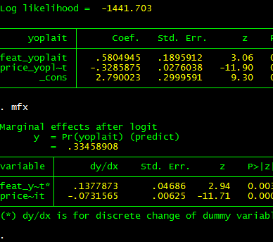
Here's the output to R's console. Note that feat.yoplait is a dummy variable for whether Yoplait had a featured advertisement that particular week. Based on my caveat, you wouldn't expect the output to be identical to Stata.



And, as you can see (compare with Stata output below), it isn't exactly the same, but if you are trying to understand the qualitative importance of your estimates, it isn't too bad.



Two bugs (quirks, kludges) remain: (1) I want to get the standard errors precisely right, (2) I want to convince mtable() to stop reporting the intercept for the marginal effects (as the intercept doesn't change, it can't have a marginal effect!). Even before I get around to this, I hope this code will have a positive marginal effect.

---

Update: The original post to which this post refers is no longer available because the TimeSeriesIreland Blog appears to have been taken down. I leave this post up subject to two caveats: (1) the standard errors are not quite right for the marginal effects and (2) the marginal effects for dummy regressors are not computed for a discrete jump from 0 to 1. Otherwise, you may find this tool useful.

Subject to the caveats in this post, if you want access to this function and a related function that is more summary()-like, I have included it in my CRAN-contributed package tonymisc (see the tab at the top of this page).

Describing Data: Frequently Used Commands

Obtaining a coherent numerical summary of data is a common task, and it is common to want to port these summary statistics into a table of results. When I am in interactive mode with my data, I use the summary() command applied to my data frame. For example, the following code loads and summarizes a data frame on Yogurt advertising and prices:

library(Ecdat) ## Econometrics Data (useful!)
data(Yogurt) ## Loads Yogurt from Ecdat
summary(Yogurt) ## Summarizes Yogurt

For each quantitative variable, the summary() command provides a five-number summary (min, max, Q1, Q3, median) plus the mean. For categorical variables, the counts of each level are provided. This provides an excellent summary measure of each variable, but you may prefer a richer set of information (especially when it comes to typing up tables).

I recently discovered a great way to obtain a richer set of information on a data frame. This method involves using the psych library, which contains functions describe() and describe.by(). Continuing with the code from above, here is the basic syntax:

library(psych)
describe(Yogurt) ## Describes in more detail the Yogurt data frame

Suppose you also want to break your summary statistics into two (or four) tables for comparison sake (perhaps to illustrate stark differences across select subsets of your data). The describe.by() command is a convenient technique to break the data down by the levels of a factor. Here's an example with on the Yogurt data.

describe.by(Yogurt, Yogurt$choice)

Finally, you may want to port your data into LaTeX format and/or select particular summary statistics from the list. I wrote a function that serves as a convenience interface to describe.by() and toLatex(). As toLatex() does not work directly on objects created using describe.by(), you might find this helpful.



If you do not like knowing about the kurtosis of your data, you could read up on the options of describe.by() to learn about how to shut it down. If you're going to port it into a LaTeX table anyway, you could also just modify the code I wrote here to eliminate the summary statistics you don't want and produce LaTeX output.

FYI: Quick R has a nice summary of some other methods for summarizing data. Of the methods at Quick R that I didn't describe, pastecs looks most like a method I would use.