Using apply() to create a unique id

Suppose you have a data set with two identifiers. For example, maybe you're studying the relationships among firms in an industry and you have a way to link the firms to one another. Each firm has an id, but the unique unit in your data set is a pairing of ids. Here's a stylized example of one such data set:


In the example that motivated this post, I only cared that A was linked with B in my data, and if B is linked with A, that's great, but it does not make A and B any more related. In other words, the order of the link didn't matter.

In this case, you'll see that our stylized example has duplicates -- id1 = "A" and id2 = "B" is the same as id1="B" and id2 = "A" for this purpose. What's a simple way to get a unique identifier? There's an apply command for that!

Thinking of each row of the identifier data as a vector, we could alphabetize (using sort(), so c("B", "A") becomes c("A", "B")), and then paste the the resulting vector together into one identifier (paste, using collapse). I call our worker function idmaker():

idmaker = function(vec){

return(paste(sort(vec), collapse=""))

}

Then, all we need to do is use the apply command to apply this function to the rows of the data, returning a vector of results. Here's how my output looks.

To get a data frame of unique links, all we need to do is cbind() the resulting vector of indices to the original data frame (and strip the duplicates). Here's some code:

co_id = apply(as.matrix(df[, c("id1", "id2")]), 1, idmaker)

df = cbind(df, co_id)

df = df[!duplicated(df[,"co_id"]),]

Here is the resulting data frame with only unique pairs.

An Application of boot() to IV regression

Bootstrapping standard errors can be a useful technique when obtaining closed form for the standard error formula is difficult or intractable. In this post, I give an example of how to use R to create a bootstrap sampling distribution in the context of IV regression. Specifically, I use boot() to automatically augment a function of mine to resample the indices of my data set with replacement (see the code in the function below).

In my application, I present a function that uses the boot library to report bootstrap standard errors for an instrumental variables regression. My ivboot() function builds on the iv() command I wrote for the tonymisc library.*

Now, onto the ivboot() example. Start by loading the tonymisc library and some data from the library, as well as the boot library.



We can run the following R script to define the function ivboot().



When applied to data and an IV regression model, the ivboot() function creates an IV regression object that -- when tonymisc is loaded -- is compatible with mtable() output. The only difference between an ivboot()-created object and an iv() object is that the ivboot() object has standard errors that are based on the bootstrap distribution of the coefficient estimates (Statistics other than the second-stage coefficient estimates are not bootstrapped).

Here is some code to compare the bootstrap output to the analytical standard error output:



On this small sample (N=100) of simulated data, the ivboot() command took less than a minute to run on my computer (timing of may vary depending on your computer). For much larger data sets, this will be slower. If you have a larger problem or lower standards (or higher standards, your choice), you can use the boots option to ivboot() to specify the number of bootstrap samples. Currently, I have set the default to 500, but you could specify boots = 200 if you want the command to run faster (boots = 10 will make it run even faster, but I don't recommend that!).

Here is the mtable() output, which can easily be ported into LaTeX using the toLatex() command.


*This standard output from an mtable() extension to my iv() command provides quite a bit of information in a convenient format. Another nice feature of iv() is that iv()-created objects have first-stage summary information readily stored in the object for extraction and analysis.

Extending mtable() to ivreg, gls and robust standard errors

I have written several extensions of the mtable() command in the memisc library that may come in handy. The methods are available in a package I have written called tonymisc (now, available on CRAN). A zipped folder with my package files is available for download here.

My extensions to mtable() allow users to easily summarize (and port into LaTeX tables) lm() objects with robust standard errors, gls() objects (created using nlme's gls) and ivreg() objects (created using AER's ivreg). If you would like to see how the output looks, here's some example code:



This code produces the LaTeX code behind this table.



I also implemented a feature through my robust() command to allow the user to select which variables he/she would like to see in the table output. Here's some example code for that feature:



The output from this code is this table:



To get this package to work for you, simply use the command install.packages("tonymisc", dependencies=TRUE), as you would normally do to install packages from CRAN. copy the tonymisc folder (available for download here) into your R library of packages. Once it is in the right place, all you need to do is load it with the library(tonymisc) command.

I am still working on the details of the package (help files, extra features, extensions of what I have done, internal consistency, loading other packages by default, ease of use, etc.), but I would be happy if people find it useful at this stage. In particular, I still need to implement some ideas from the comments (the next version will contain these). If you have other suggestions, please leave a comment to let me know.

Putting Robust Standard Errors into LaTeX Tables: An Extension of mtable

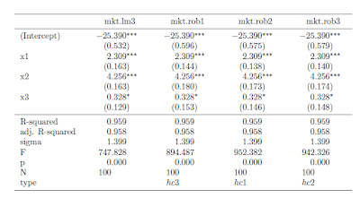
I recently discovered the mtable() command in the memisc library and its use with toLatex() to produce nice summary output for lm and glm objects in a nicely formatted table like this:



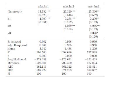
Once you have your linear model objects, all you need is one command -- a composite of toLatex() and mtable(). Here's the R code I used to generate the LaTeX code:



All you need to do from here is to copy the code into your LaTeX document (or in my case LyX document with evil red text), where you use the dcolumn and booktabs packages (specify this in the preamble using \uspackage{} for each package).

This is really straightforward ... as long as you just want to use lm or glm objects with no deviations from that baseline. But, what if you -- as many econometricians do -- want to estimate your linear model with heteroskedasticity-consistent standard errors?

How to do it with "robust" standard errors

My favorite way to robustify my regression in R is to use some code that John Fox wrote (and I found in an R-help forum). He called it summaryHCCM.lm(). In my own applications, I have renamed it summaryR() because "R" makes me think "robust" and it is fewer keystrokes than HCCM. I modified the output of the code to work better with what follows:



Suppose I would like to produce nicely-typed output like the above table, but with robust standard errors. Unfortunately, the summaryR() solution doesn't map naturally into our mtable() solution to producing nice LaTeX output. But, fortunately, there is a solution.

(If you just want this to work, copy and run all of the code from here to "so we are all set." No need to understand the implementation details. If you're interested in understanding how I arrived at my solution, here come the details)

It turns out that there is a way to map the summaryR() command to the mtable() command to produce nice LaTeX output with robust standard errors. Once we have the commands, the syntax is just as easy as using summaryR() directly and it makes creating LaTeX table output easy. So, what do we do?

First, we need to adapt the methods behind mtable() to allow it to recognize something that I call a "robust" object. To do this, we need to write a function called getSummary.robust()



and we need to set some formatting options using the setSummaryTemplate() command:



Second, we need to convert a linear models object into something called a "robust" object. The robust() command does this:



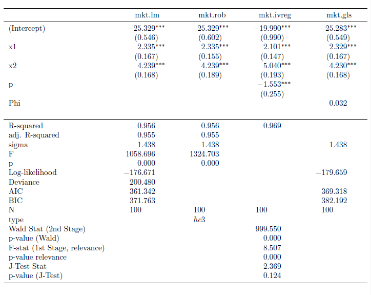
So, we are all set. If you run all of the preliminary code in this post, you're in good shape to produce LaTeX tables with robust standard errors like this table:



Once the functions are defined, the syntax is straightforward. Here is the code I used to put together the the table (plus, one step to copy the output into my LyX file)



I hope this is helpful. If you're interested in other extensions of mtable(), here's an excellent post.

Finally, I am still learning I learned how to bundle functions into a package (so I haven't made this available as a package yet). Today, I was able to successfully package this set of functions into a package called tonymisc on my computer. Once I organize the help/example/other fun parts of the package, I will see about making this and my extension for ivreg objects available. This package (in its first version) is available on CRAN through install.packages("tonymisc").

Forming Formulas

One of the first functions a new R user learns how to use is the lm() command, which involves stating the model formula.

lm(y~x1+x2, data=mydata)

After a while, this just becomes a natural way to say "I want a regression of y on x1 and x2 using mydata." Even though it is natural, the underlying structure of the formula is not as it first appears. This becomes apparent as soon as you need to work with formula objects when writing your own function.

Does ~ define a string? No. You can ask R directly whether the formula is a string (of class "character") using is.character().

is.character(y~x1+x2+x3)
[1] FALSE

As we will soon see, a formula isn't easily coerced into a string either.

Should we think of ~ as a fancy = sign? No. R doesn't think of ~ as defining an equation to be evaluated.

x1=5
x2=6
x3=7
y~x1+x2+x3
y ~ x1 + x2 + x3

It is better to think of ~ as defining the entire statement as an object with a special class called formula, which conveys the idea of the model to other functions in R.

For the rest of the post, I will show some calculations that illustrate more fundamentally what a formula object is.  For concreteness, imagine you have a formula object with the general form y~x1+x2+z1+z2+z3.

You could define this object with the command:

form.ex = y~x1+x2+z1+z2+z3
Suppose our goal is to extract the first two explanatory variables (x1 and x2) and use them in a linear model for the response (y).  If you're reading this for help, you likely have a more noble goal in mind.  Take this as an illustrative example.

To appreciate the power of a method, it is useful to see the inelegant code we are avoiding.  The inelegant code also shines some light on how a formula object differs from a string.

An inelegant method

We could gain access to the elements of the formula by coercing it into a character string using as.character().  If we do this in our example, we obtain a character vector of length three:

as.character(form.ex)
[1] "~"                 
[2] "y"                 
[3] "x1 + x2 + z1 + z2 + z3"
Here, we see that the RHS of the formula is stored in the third element of this vector.  The response is in the second element of the vector.  Let's store these into vectors we can easily reference and use.

rhs= as.character(form.ex)[3]
resp = as.character(form.ex)[2]

Next, we can splice the rhs vector to obtain the individual variable names using the strsplit command.  Note: we want to split the vector apart using a delimiter " + " with the spaces.  Because the + is an operator, we need to use " \\+ " instead.  In addition, strsplit() returns a list of length two.  We really want the first element of the list... (remember, this is the inelegant way).

rhs.sp = strsplit(rhs," \\+ ")[[1]]
rhs.sp
[1] "x1" "x2" "z1" "z2" "z3"
Now, we have a vector of variable names for the right hand side of the equation.  As our goal is to construct a formula object relating the response to the first two explanatory variables, extract the first two elements of this vector.

rhs.new= rhs.sp[1:2]
rhs.new
[1] "x1" "x2"
And, paste this right hand side of the equation to the response variable name in a formula style using the following combination of paste() commands.

short.form=paste(resp,"~",paste(rhs.new,collapse="+"))
short.form
[1] "y ~ x1+x2"
Great.  The only problem?  The object short.form is not a formula object.  It is a character string.  This won't be a problem if we input it into something like lm(), which will coerce it to a formula object before using it.

lm(short.form, data=mkt.df)

Call:
lm(formula = short.form, data = mkt.df)

Coefficients:
(Intercept)           x1           x2
-25.329        2.335        4.239  
If you want to do the formula coercion yourself, you can use the as.formula() command as follows.

short.form=as.formula(short.form)
short.form
y ~ x1 + x2
A more elegant method

The all.vars() command does the splitting, splicing and extracting that comprised the bulk of what we did above.  Starting with the formula object form.ex, we could create a vector of variable names in our model statement as:

vars.ex = all.vars(form.ex)
vars.ex
[1] "y"  "x1" "x2" "z1" "z2" "z3"
Now, just define the rhs and resp vectors as we did in the less elegant method.

rhs = vars.ex[2:3]
resp   = vars.ex[1]
Is there a better way recombine these vectors than to create our own paste collapser?  Yes!  The reformulate() function makes it easy.

myform=reformulate(rhs.av, response=resp)
myform
y ~ x1 + x2
And, for good measure, let's see what happens in the lm() command:

lm(myform, data=mkt.df)

Call:
lm(formula = myform, data = mkt.df)

Coefficients:
(Intercept)           x1           x2
-25.329        2.335        4.239

Dates in R and the First Day of the Month

I spent some time this morning learning about how R thinks about dates in R. I found this website to be a useful guide.

Imagine that your data are dates in a standard format [YEAR-MONTH-DAY (as in 2011-23-04) is one such format] and you want a vector of the dates that are the first day in the month of your data set. You might, for example, be interested in this (as an intermediate calculation) because you wish to match some S&P 500 returns data to monthly data. Frustratingly, the S&P 500 returns data do not report on the weekends or on holidays when the exchange is closed.

Here's a function that will do return a vector of first-days-of-the-month if you give it a vector of dates. Maybe you will find this useful.



Enjoy!