Defaults, Lists and Classes: A Functional Post

In this post, I demonstrate a couple of useful tricks to writing functions in R. The context is a function I wrote called called samp() that allows for an easy demonstration of sampling distribution properties.



Defaults

By default, this function draws K = 500 samples of size N from a normal distribution with a mean of mu = 0 and a standard deviation of std = 1. As you can see, the syntax for specifying a default for an argument to the function is to set it equal to its default value inside the function statement. Arguments can be given no default by naming them as an argument to the function without specifying their default value.

Sensibly chosen defaults can save a lot of time for people who use your function. For example, although this samp() function has four arguments, I don't need to type samp(100, 0, 1, 500) every time I wish to take 500 samples of size N=100 from a Normal(0,1) random variable. If sampling from a Normal(0,1) is especially common, setting the defaults this way can save a lot of keystrokes.

On the other hand, using defaults instead of hard coding the Normal(0,1) choice has the distinct advantage that users get flexibility from your function giving them the option to specify arguments other than the default. The right use of defaults strikes the perfect balance between ease of use and flexibility.

Returning a List... with Names

If your function warrants the special treatment, you have probably performed several useful calculations that you would like to return. Maybe you have conducted several related hypothesis tests that you would like to reference later (report and/or use in another calculation). A great way to do this is to store the results of your function into a list.

For example, in the samp() function, I wanted to store vectors of the sample means, sample standard deviations and standard errors (500, one for each replication). For good measure, I wrote the function to store the means and standard deviations of these vectors as well as the true parameter values that went into the function.

Although it is often a good idea to store the results in a list, it is a better idea to name the elements of the list for easy extraction. If I ran the command

mysamp = samp(100)

The object mysamp would contain a list of the results from the function samp(). Suppose I want to extract the vector of means (for example, to compute a histogram). Without running the names command, I would have to remember that the vector of means was in the first position in the list and use the command

hist(mysamp[1])

to plot a histogram of the means vector from my sampling object. As it is easy to forget the precise order in which the elements of a function are stored, this syntax can lead to too much thinking. It is better to name the first list element something like means. Naming the list elements allows the user to use the $ extractor on objects created with the function. That is, the syntax becomes

hist(mysamp$means)

which is much easier to remember and easier to read. This latter fact is often unappreciated, but if you get in the habit of naming elements in a list, you will be a better collaborative coder. Even if you're not into collaboration, when you return to that project after two weeks of doing something else, it is much easier to remember where you left off.

A Benefit of Keeping It Classy

Another coding practice that often goes unappreciated is the use of classes to make your life easier (and your console cleaner). At this point, if you type mysamp into your console window, R will bombard you with more than a screen's worth of output. Most of this is output that I don't want to see printed out. I might want to save it for later, but I don't want to save it.

This is where the class(result) = "samp" command comes in handy. By "classing" my object this way and writing a short a print method for this class (named print.samp()), I can cut down on the amount of output I have to see when I inspect my object. Here's code to define a print method.



Now, try typing mysamp into R. You will see much less output (only the output from print.samp), but the object mysamp still has all of the information you want to keep around. If you don't believe me, just type mysamp$means to be sure.

Just as we could "class and print," we can also "class and plot." This can be handy if you want there to be a standard meaning for the command plot(mysamp). In our working example, let's make this command mean plot three histograms, one for means, one for standard deviations and one for standard errors. Here's some code that imposes this meaning on objects with class "samp"



In case you were wondering what this plotting out looks like, here is the picture that is produced from the command plot(mysamp).

Porting Stata-like Marginal Effects to LaTeX

The TimeSeriesIreland Blog posted an excellent start on a function that automatically computes marginal effects for probit and logit models. As I have always wanted an easy-to-use function that computes and reports marginal effects in R, I was elated to see the function and I couldn't wait to use it.

My initial impression when I saw the post was: "I should write an mtable() extension for that to go with my other extensions." With this in mind, I started familiarizing myself with the code and I contacted the author to make sure he was fine with me extending his code (and adding it to my package with mtable() extensions). As he was fine with my goal of extending the function, here is a post where I introduce you to a new extension to mtable().

Important Caveat: At this point, the function does not do the technically "right" thing (delta method) to obtain the standard errors on the marginal effects. Instead, it supposes that the z-score will remain constant across the transformation, which isn't quite right. Even though it isn't perfect, in most of the examples I have tried, the results are almost identical to Stata output. You tend to get more divergence from the Stata solution for dummy variable regressors (where Stata computes a discrete jump rather than a derivative).

One would think that an extension of mfx() would use mfx(), but that didn't turn out to be the easy way to go. After many unsuccessful attempts (more about this in a future post; I learned some things worth sharing), here's the solution I landed on.

First, define an "mfx" object with a function that changes the class attribute of a fitted glm object to. Here's code to define a function to do this.



Second, make sure you have the memisc library loaded with the command library(memisc) -- or library(tonymisc), which loads memisc among other excellent packages.

Third, until I get the kinks worked out and port this into my package, you'll have to run code to define a getSummary.mfx() method to extend mtable. Here's some code that will do this.



Now, I suppose you want to know how this extension works. Here's an example that uses some data from the wonderful Ecdat library (a great source for Econometrics data sets).



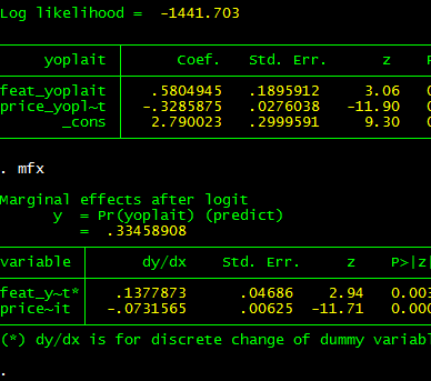
Here's the output to R's console. Note that feat.yoplait is a dummy variable for whether Yoplait had a featured advertisement that particular week. Based on my caveat, you wouldn't expect the output to be identical to Stata.



And, as you can see (compare with Stata output below), it isn't exactly the same, but if you are trying to understand the qualitative importance of your estimates, it isn't too bad.



Two bugs (quirks, kludges) remain: (1) I want to get the standard errors precisely right, (2) I want to convince mtable() to stop reporting the intercept for the marginal effects (as the intercept doesn't change, it can't have a marginal effect!). Even before I get around to this, I hope this code will have a positive marginal effect.

---

Update: The original post to which this post refers is no longer available because the TimeSeriesIreland Blog appears to have been taken down. I leave this post up subject to two caveats: (1) the standard errors are not quite right for the marginal effects and (2) the marginal effects for dummy regressors are not computed for a discrete jump from 0 to 1. Otherwise, you may find this tool useful.

Subject to the caveats in this post, if you want access to this function and a related function that is more summary()-like, I have included it in my CRAN-contributed package tonymisc (see the tab at the top of this page).

Describing Data: Frequently Used Commands

Obtaining a coherent numerical summary of data is a common task, and it is common to want to port these summary statistics into a table of results. When I am in interactive mode with my data, I use the summary() command applied to my data frame. For example, the following code loads and summarizes a data frame on Yogurt advertising and prices:

library(Ecdat) ## Econometrics Data (useful!)
data(Yogurt) ## Loads Yogurt from Ecdat
summary(Yogurt) ## Summarizes Yogurt

For each quantitative variable, the summary() command provides a five-number summary (min, max, Q1, Q3, median) plus the mean. For categorical variables, the counts of each level are provided. This provides an excellent summary measure of each variable, but you may prefer a richer set of information (especially when it comes to typing up tables).

I recently discovered a great way to obtain a richer set of information on a data frame. This method involves using the psych library, which contains functions describe() and describe.by(). Continuing with the code from above, here is the basic syntax:

library(psych)
describe(Yogurt) ## Describes in more detail the Yogurt data frame

Suppose you also want to break your summary statistics into two (or four) tables for comparison sake (perhaps to illustrate stark differences across select subsets of your data). The describe.by() command is a convenient technique to break the data down by the levels of a factor. Here's an example with on the Yogurt data.

describe.by(Yogurt, Yogurt$choice)

Finally, you may want to port your data into LaTeX format and/or select particular summary statistics from the list. I wrote a function that serves as a convenience interface to describe.by() and toLatex(). As toLatex() does not work directly on objects created using describe.by(), you might find this helpful.



If you do not like knowing about the kurtosis of your data, you could read up on the options of describe.by() to learn about how to shut it down. If you're going to port it into a LaTeX table anyway, you could also just modify the code I wrote here to eliminate the summary statistics you don't want and produce LaTeX output.

FYI: Quick R has a nice summary of some other methods for summarizing data. Of the methods at Quick R that I didn't describe, pastecs looks most like a method I would use.

Extending mtable() to ivreg, gls and robust standard errors

I have written several extensions of the mtable() command in the memisc library that may come in handy. The methods are available in a package I have written called tonymisc (now, available on CRAN). A zipped folder with my package files is available for download here.

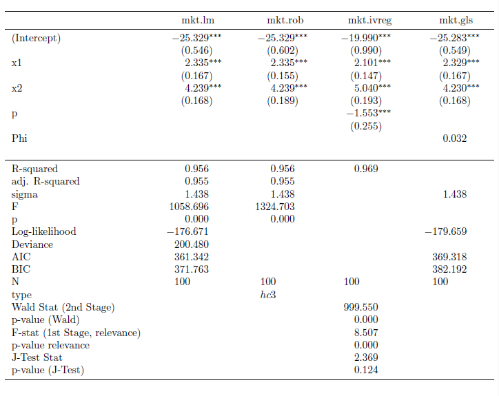
My extensions to mtable() allow users to easily summarize (and port into LaTeX tables) lm() objects with robust standard errors, gls() objects (created using nlme's gls) and ivreg() objects (created using AER's ivreg). If you would like to see how the output looks, here's some example code:



This code produces the LaTeX code behind this table.



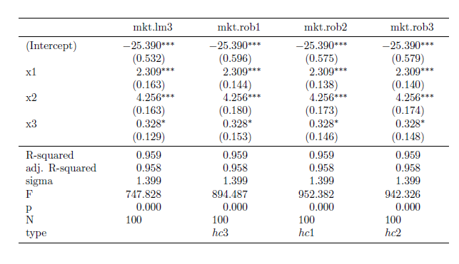
I also implemented a feature through my robust() command to allow the user to select which variables he/she would like to see in the table output. Here's some example code for that feature:



The output from this code is this table:



To get this package to work for you, simply use the command install.packages("tonymisc", dependencies=TRUE), as you would normally do to install packages from CRAN. copy the tonymisc folder (available for download here) into your R library of packages. Once it is in the right place, all you need to do is load it with the library(tonymisc) command.

I am still working on the details of the package (help files, extra features, extensions of what I have done, internal consistency, loading other packages by default, ease of use, etc.), but I would be happy if people find it useful at this stage. In particular, I still need to implement some ideas from the comments (the next version will contain these). If you have other suggestions, please leave a comment to let me know.

Putting Robust Standard Errors into LaTeX Tables: An Extension of mtable

I recently discovered the mtable() command in the memisc library and its use with toLatex() to produce nice summary output for lm and glm objects in a nicely formatted table like this:



Once you have your linear model objects, all you need is one command -- a composite of toLatex() and mtable(). Here's the R code I used to generate the LaTeX code:



All you need to do from here is to copy the code into your LaTeX document (or in my case LyX document with evil red text), where you use the dcolumn and booktabs packages (specify this in the preamble using \uspackage{} for each package).

This is really straightforward ... as long as you just want to use lm or glm objects with no deviations from that baseline. But, what if you -- as many econometricians do -- want to estimate your linear model with heteroskedasticity-consistent standard errors?

How to do it with "robust" standard errors

My favorite way to robustify my regression in R is to use some code that John Fox wrote (and I found in an R-help forum). He called it summaryHCCM.lm(). In my own applications, I have renamed it summaryR() because "R" makes me think "robust" and it is fewer keystrokes than HCCM. I modified the output of the code to work better with what follows:



Suppose I would like to produce nicely-typed output like the above table, but with robust standard errors. Unfortunately, the summaryR() solution doesn't map naturally into our mtable() solution to producing nice LaTeX output. But, fortunately, there is a solution.

(If you just want this to work, copy and run all of the code from here to "so we are all set." No need to understand the implementation details. If you're interested in understanding how I arrived at my solution, here come the details)

It turns out that there is a way to map the summaryR() command to the mtable() command to produce nice LaTeX output with robust standard errors. Once we have the commands, the syntax is just as easy as using summaryR() directly and it makes creating LaTeX table output easy. So, what do we do?

First, we need to adapt the methods behind mtable() to allow it to recognize something that I call a "robust" object. To do this, we need to write a function called getSummary.robust()



and we need to set some formatting options using the setSummaryTemplate() command:



Second, we need to convert a linear models object into something called a "robust" object. The robust() command does this:



So, we are all set. If you run all of the preliminary code in this post, you're in good shape to produce LaTeX tables with robust standard errors like this table:



Once the functions are defined, the syntax is straightforward. Here is the code I used to put together the the table (plus, one step to copy the output into my LyX file)



I hope this is helpful. If you're interested in other extensions of mtable(), here's an excellent post.

Finally, I am still learning I learned how to bundle functions into a package (so I haven't made this available as a package yet). Today, I was able to successfully package this set of functions into a package called tonymisc on my computer. Once I organize the help/example/other fun parts of the package, I will see about making this and my extension for ivreg objects available. This package (in its first version) is available on CRAN through install.packages("tonymisc").

Forming Formulas

One of the first functions a new R user learns how to use is the lm() command, which involves stating the model formula.

lm(y~x1+x2, data=mydata)

After a while, this just becomes a natural way to say "I want a regression of y on x1 and x2 using mydata." Even though it is natural, the underlying structure of the formula is not as it first appears. This becomes apparent as soon as you need to work with formula objects when writing your own function.

Does ~ define a string? No. You can ask R directly whether the formula is a string (of class "character") using is.character().

is.character(y~x1+x2+x3)
[1] FALSE

As we will soon see, a formula isn't easily coerced into a string either.

Should we think of ~ as a fancy = sign? No. R doesn't think of ~ as defining an equation to be evaluated.

x1=5
x2=6
x3=7
y~x1+x2+x3
y ~ x1 + x2 + x3

It is better to think of ~ as defining the entire statement as an object with a special class called formula, which conveys the idea of the model to other functions in R.

For the rest of the post, I will show some calculations that illustrate more fundamentally what a formula object is.  For concreteness, imagine you have a formula object with the general form y~x1+x2+z1+z2+z3.

You could define this object with the command:

form.ex = y~x1+x2+z1+z2+z3
Suppose our goal is to extract the first two explanatory variables (x1 and x2) and use them in a linear model for the response (y).  If you're reading this for help, you likely have a more noble goal in mind.  Take this as an illustrative example.

To appreciate the power of a method, it is useful to see the inelegant code we are avoiding.  The inelegant code also shines some light on how a formula object differs from a string.

An inelegant method

We could gain access to the elements of the formula by coercing it into a character string using as.character().  If we do this in our example, we obtain a character vector of length three:

as.character(form.ex)
[1] "~"                 
[2] "y"                 
[3] "x1 + x2 + z1 + z2 + z3"
Here, we see that the RHS of the formula is stored in the third element of this vector.  The response is in the second element of the vector.  Let's store these into vectors we can easily reference and use.

rhs= as.character(form.ex)[3]
resp = as.character(form.ex)[2]

Next, we can splice the rhs vector to obtain the individual variable names using the strsplit command.  Note: we want to split the vector apart using a delimiter " + " with the spaces.  Because the + is an operator, we need to use " \\+ " instead.  In addition, strsplit() returns a list of length two.  We really want the first element of the list... (remember, this is the inelegant way).

rhs.sp = strsplit(rhs," \\+ ")[[1]]
rhs.sp
[1] "x1" "x2" "z1" "z2" "z3"
Now, we have a vector of variable names for the right hand side of the equation.  As our goal is to construct a formula object relating the response to the first two explanatory variables, extract the first two elements of this vector.

rhs.new= rhs.sp[1:2]
rhs.new
[1] "x1" "x2"
And, paste this right hand side of the equation to the response variable name in a formula style using the following combination of paste() commands.

short.form=paste(resp,"~",paste(rhs.new,collapse="+"))
short.form
[1] "y ~ x1+x2"
Great.  The only problem?  The object short.form is not a formula object.  It is a character string.  This won't be a problem if we input it into something like lm(), which will coerce it to a formula object before using it.

lm(short.form, data=mkt.df)

Call:
lm(formula = short.form, data = mkt.df)

Coefficients:
(Intercept)           x1           x2
-25.329        2.335        4.239  
If you want to do the formula coercion yourself, you can use the as.formula() command as follows.

short.form=as.formula(short.form)
short.form
y ~ x1 + x2
A more elegant method

The all.vars() command does the splitting, splicing and extracting that comprised the bulk of what we did above.  Starting with the formula object form.ex, we could create a vector of variable names in our model statement as:

vars.ex = all.vars(form.ex)
vars.ex
[1] "y"  "x1" "x2" "z1" "z2" "z3"
Now, just define the rhs and resp vectors as we did in the less elegant method.

rhs = vars.ex[2:3]
resp   = vars.ex[1]
Is there a better way recombine these vectors than to create our own paste collapser?  Yes!  The reformulate() function makes it easy.

myform=reformulate(rhs.av, response=resp)
myform
y ~ x1 + x2
And, for good measure, let's see what happens in the lm() command:

lm(myform, data=mkt.df)

Call:
lm(formula = myform, data = mkt.df)

Coefficients:
(Intercept)           x1           x2
-25.329        2.335        4.239

Automatically Save Your Plots to a Folder

Suppose you're working on a problem that involves a loop for calculations. At each iteration inside the loop, you want to construct a plot. Not only do you want to see the plot, but you would like to save each plot for a presentation, report or paper. Furthermore, the loop goes on for a while (say through the 26-letters of the alphabet).

The last thing you want to do in this situation is: (1) produce each plot one-by-one, (2) right click on each singly-produced plot to save, (3) give the plot a unique name, and (4) repeat. You'll spend too much of your time saving plots and not enough time thinking about whether they are the right plots. Just imagine, what if something went wrong and you need to produce the whole set of plots again?

RStudio has a nice feature in that it saves all of your plots in the plotting pane. It's no problem if you just produce the plot inside your dreaded loop in RStudio because it keeps all of your plots in the pane. Even with RStudio, if you produce the plots inside the loop, you still need to save each one individually. This isn't ideal. If you don't believe me, imagine that you have 1000 plots instead of 26. This manual-saving method becomes impractical quickly.

How then can you automatically save plots to a folder without spending too much time? That's today's task. I'll start by describing several building-block commands and then at the end I'll put together a loop that does it all (by way of contrived example).

The first command you need to know is jpeg() (Alternatively, bmp(), png() or tiff(), depending on your file-type preferences) paired with dev.off(). For our purposes, jpeg() takes a path argument that allows us to save (at the location of our choosing via the path) output to a plotting window. For example, this code will save the next plotting object to a jpeg file called myplot.jpg located at "C://R//SAVEHERE"

jpeg(file = "C://R//SAVEHERE//myplot.jpg")

After running the plotting object, you need to be sure to turn off the plotting device you created (with the jpeg() command). To save a scatter plot of the vectors x versus y to the location described above, run these three lines:

jpeg(file = "C://R//SAVEHERE//myplot.jpg")
plot(x,y)
dev.off()

This code is a good building block for automatically saving to a folder inside a loop, but we still need to know how to dynamically create file names at which to save our plots. Suppose we have a vector that gives us a list of identifiers called names. Presumably, these identifiers mean something in your setting. For our working example, names is a list of letters from A to Z (we are trying to produce a separate scatter plot for each letter from A to Z).

We can use the file.path() and paste() commands to help us out here. I have found paste() to be incredibly useful for other applications as well. For example,

paste("myplot_", i, ".jpg", sep="")

produces the character string myplot_50.jpg when i = 50 and myplot_51.jpg when i=51. If i changes for each iteration in the loop, this paste() command will create a unique file name at each iteration.

We can get fancier with our pasting. If we have a vector of names, we can extract the ith name from the names vector with the paste command:

paste("myplot_", names[i], ".jpg", sep="")

The file.path() function helps us in a different way. It is a special paste function that helps us construct file paths really easily. For example,

mypath=file.path("C:", "R", "SAVEHERE", filename)

returns "C://R//SAVEHERE//filename" and stores it in an object called mypath. Replace filename with the paste command and we have a way to automatically generate file names in a folder called SAVEHERE.

Now, you have the tools to understand my example code of how to automatically generate and save plots to a folder. Make sure the folder exists before saving, but subject to that constraint, this procedure may make your life easier.