Using apply() to create a unique id

Suppose you have a data set with two identifiers. For example, maybe you're studying the relationships among firms in an industry and you have a way to link the firms to one another. Each firm has an id, but the unique unit in your data set is a pairing of ids. Here's a stylized example of one such data set:


In the example that motivated this post, I only cared that A was linked with B in my data, and if B is linked with A, that's great, but it does not make A and B any more related. In other words, the order of the link didn't matter.

In this case, you'll see that our stylized example has duplicates -- id1 = "A" and id2 = "B" is the same as id1="B" and id2 = "A" for this purpose. What's a simple way to get a unique identifier? There's an apply command for that!

Thinking of each row of the identifier data as a vector, we could alphabetize (using sort(), so c("B", "A") becomes c("A", "B")), and then paste the the resulting vector together into one identifier (paste, using collapse). I call our worker function idmaker():

idmaker = function(vec){

return(paste(sort(vec), collapse=""))

}

Then, all we need to do is use the apply command to apply this function to the rows of the data, returning a vector of results. Here's how my output looks.

To get a data frame of unique links, all we need to do is cbind() the resulting vector of indices to the original data frame (and strip the duplicates). Here's some code:

co_id = apply(as.matrix(df[, c("id1", "id2")]), 1, idmaker)

df = cbind(df, co_id)

df = df[!duplicated(df[,"co_id"]),]

Here is the resulting data frame with only unique pairs.

Splitting Vectors of Uneven Strings

Suppose you have a vector of names such that the first three words in the vector contain relevant information, but there is a bunch of extraneous stuff. For example,



Our goal is to collapse the first three words into one contiguous string (without the spaces) and we want to discard the extra words (because they're extraneous infromation). For a situation like this, my first thought is to use the strsplit() command, which splits vectors of strings by any specified character pattern you wish. For example, suppose that an object named myvec contains the vector of strings we would like to split into separate words. Then, the command

strsplit(myvec, " ")

produces a list of vectors of words. This is a little cumbersome because the vectors have a different length for each element in the list. Fortunately, all we want in this application is the first three words concatenated together, so some trimming will still give us the right answer. Even better, if you don't mind seeing an error message on account of trying to bind vectors of uneven lengths, we can rbind the list together using do.call() as follows:

do.call(rbind, strsplit(myvec, " "))

This still works because R recycles. For our example, we then obtain a fabulous 4x5 matrix of names:



Store this matrix in the object namemat, then reduce this matrix to containing only the first three words by selecting those columns:

namemat = namemat[, 1:3]

Think of each row of this resulting matrix as a vector. If we can paste this vector together into one string, we're done. Do this using the paste() command with collapse = "". To paste() simultaneously for each row, I like to use apply. The resulting command that goes from namemat to vector of cleaned-and-concatenated strings is:

apply(namemat, MARGIN = 1, FUN = function(x){ paste(x, collapse="")})

MARGIN = 1 is for rows. Putting the pieces together, the code we developed is:

namemat = do.call(rbind, strsplit(myvec, " "))
namemat = namemat[, 1:3]
apply(namemat, MARGIN = 1, FUN = function(x){ paste(x, collapse="")})

And, this should work if your list of names is 4 lines long or 40 million lines long. That said, there was a lot of heavy lifting along the way (we created a list, collapsed a list, produced an error message as a byproduct of binding the list into a matrix, pasted each row using the collapse option and pasted quickly using apply).

There's a strange way to do this same task that doesn't require the same heavy lifting (just different heavy lifting). Use write.table() and read.table(). Start by writing the unclean initial vector to a text file without row names.

write.table(myvec, "C://vec.txt", sep = "", quote = FALSE, row.names = FALSE)

Also, turn off quoting. We do this to trick R into thinking that the spaces we want to eliminate are space delimiters. Then, read in the file using read.table() and a space delimiter.

namemat = read.table("Data/Raw/crspnames.txt", skip=1, sep = " ", quote = "", fill = TRUE)

skip =1 is to avoid reading in the variable name. The fill = TRUE argument fills in the matrix so that read.table() doesn't return an error for trying to read a non-square table. Each row of the resulting matrix namemat has a full name to be collapsed, one word per column (similar to namemat from the previous method). To complete the task, we still need to paste the first three columns together for each row. For this, use the apply-the-paste technique we used in the first method.

On a final note, if we don't mind pasting the entire vector together without the spaces (including the extraneous stuff), the easy solution is to use the gsub() command to replace spaces with nothing.

gsub(" ", "", myvec)

This method will produce an answer that is close to the one that we wanted and with a simple one line of code. Depending on your objective, this may be the best way to go -- that is, if you don't care about having extra words appended to each string.

Avoiding Loops in R: An Example with Principal Minors

Yesterday, I found myself wanting to compute a large subset of the second order principal minors of a matrix (diagonal-preserving minors; the ones for which the rows and columns kept are the same). Don't judge me for wanting to do this, and bear with me, there is a lesson about R programming here (mostly for me, read the comments for testing).

If you don't know what a principal minor is or forgot what it was (because most of us don't spend much time with principal minors), here is a short refresher on how to get a second-order principal minor (other orders are possible and there's a lot of related theory, but let's try to focus on this one task for now).

Step 1: Deletion. Take any matrix. Delete all but two rows and all but two columns. For example, suppose the matrix is 5x5 and let's keep rows 1 and 3 and columns 2 and 4 (lots of other combinations are possible).

In the back of your mind, think how easy this is in R.

Step 2: Calculation. Once we delete the irrelevant parts of the big matrix to get our 2x2 submatrix, obtain the principal minor by taking the determinant of the resulting 2x2 matrix. For our example, we compute 3x2 - 3x1 = 3.

Both steps in this calculation are easy to implement in R. For the first step, merely use R's fantastic syntax for extracting rows and columns of matrices. If the matrix is called mat, we efficiently perform the first step by:

little_mat = mat[c(1,3), c(2,4)]

That's easy enough. With little_mat in hand, the second step is even easier.

pm = det(little_mat)

The real trick to this programming problem is picking out all of principal minors I want to compute (diagonal-preserving ones that keep the same-numbered rows and columns; little_mat won't do because c(1,3) is not c(2,4)), and doing it efficiently. I also don't want to rewrite my code as my matrix changes size.

So, what do we do? A really bad An idea that will eventually compute the right answer is to write this using for() loops.




Barring a coding error, this code should eventually work, but it will be slow (or fast depending on how you write it). If you want to run through this code many times (like I did yesterday), efficiency is at a premium and you should immediately think of faster techniques -- like using the apply() function (or preallocating your storage vector, which actually saves time).

Before moving to apply(), we need a quick way to enumerate all of the ways to keep two out of N rows. If we were counting, that's N choose 2, also known as a combination. Fortunately, this step has already been implemented in the gregmisc library with a function called combinations(). Conveniently, combinations(N, 2) will return a matrix with all of the ways to select two numbers less than or equal to N as its rows. There are other options, but this is the default, which is perfect for our application.

For example, here is some output for N=5.


With this way of computing the rows/ columns we want to keep, all we need to do is put our simple code for computing a second order principal minor into a function. Let's call it minor2(). Then, use apply() to apply this function to each row (MARGIN=1 is for rows) of the combinations matrix. Here's the complete set of code that will work if you have a matrix called mat for which you want the diagonal-second order principal minors.



Because we avoid doing loops, this method is much faster. For a big project, this added efficiency is worth it. More generally, this technique of using apply() to avoid repeatedly looping is a good lesson to apply to other programming problems.

Update: Thanks to Berend for going through the trouble of system.time() testing the code in this post (and spiceman for a good comment as well). Read on into the comments for more, but for a preview of what we learned: (1) The copying via c() is what slows the loop down, (2) apply is slightly slower than writing the loop yourself, (3) combn(), the combinations() alternative, is really slow, and (4) one should always stand behind system.time() methods before talking about the efficiency of a method.

I much appreciate the feedback. One of the reasons I have this blog is to learn more about R (and those comments were definitely informative).

Today's Assignment: Assignment

A new R user quickly discovers that there are multiple ways to store information into an object -- the technical term for this is assignment. There's = as in:

x = c(1,2,3)

and there's <- as in:

x <- c(1,2,3)

R help on assignOps offers this explanation of the difference:

The operators <- and = assign into the environment in which they are evaluated. The operator <- can be used anywhere, whereas the operator = is only allowed at the top level (e.g., in the complete expression typed at the command prompt) or as one of the subexpressions in a braced list of expressions.

For catching subtle coding errors with =, this is a smart feature of R. When I am tired, I sometimes find myself writing a line of code that looks like this:

if(codename = "thedoctor") watch = "yes"

In this line of code, the problem is that codename = "thedoctor" isn't a logical statement. It is a statement that would assign the string "thedoctor" to an object called codename.... if the statement were allowed by R's language. Fortunately, R prevents this.

This feature of the R programming language helps me because I -- by default -- use = for assignment rather than <-. My style is not conventional, however. Popular R coding style guides (Google, 4D pie charts) suggest that users use <- option for assignment, rather than =.

Deep down, I think I use this unconventional default because I had the = versus == distinction (more generally, assignment versus logical statement) drilled into me in my first computer science class (not in R; Java). On reflection, I have three reasons to use = rather than <-. First, = is easier to type, using one keystroke and no shift keys. Second, the equals style looks cleaner to me (completely a personal preference). Third, I think assignment should take place out in the open (i.e., exactly where = is allowed). If the line of code is out in the open, both <- and = work the same.

On a final note, the <- is not without its problems for logical statements. For example, the statement

if(agediff<-2) status = "I'm older"

will cause problems and it won't let you know about these problems until you get some really strange results later on. Here's the code from an interactive R session where I show what can go wrong.

> agediff = -3
> if(agediff<-2) status = "I'm older"
> status
[1] "I'm older"
> agediff
[1] 2
> agediff = 4
> if(agediff<-2) status = "I'm older"
> status
[1] "I'm older"
> agediff
[1] 2
> status=NULL
> if(agediff<-2) status = "I'm older"
> status
[1] "I'm older"
> agediff
[1] 2

The problem is two-fold in this code. First, the if statement isn't acting as a logical statement splitting by whether "agediff< -2" Second, the value of agediff is changed because "<-" means assignment. The result is that both status and agediff have (potentially) the wrong values at the end of running the code.

As this error is a problem whether you use = or <- for assignment, it is worth knowing regardless of your style preference. Adhering to good spacing guidelines is a good way to avoid this error.

> agediff = 4
> if(agediff < -2) status = "I'm older"
> status
NULL
> agediff
[1] 4

There are some other examples in the Stack Overflow forum discussion on this topic (actually multiple threads on this), all of which are useful. It is interesting reading to be sure.

An application of aggregate() and merge()

Today, I encountered an interesting problem while processing a data set of mine. My data have observations on businesses that are repeated over time. My data set also contains information on longitude and latitude of the business location, but unfortunately, my source only started providing the longitude and latitude information in the middle of the data set. As a result, the information is missing for the first few periods for every business, but across businesses, I have latitude and longitude information for virtually all of my data set.

As long as the business hasn't shifted location, this isn't a problem. I can just substitute the lat-long information from the later periods into the earlier periods for each business. This sounds simple enough to do, but when one has a data set with 70,000 observations, an automatic process saves a lot of time and can help avoid mistakes.

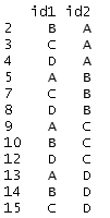
Let's start by building common ground. Here is a script that you can use to simulate a data set to follow along.



Once you run this script, the data frame mydat is a balanced panel of 125 businesses observed over 25 time periods (my actual data set is an unbalanced panel and the solution I present works just as well for unbalanced as with balanced. It is just easier to simulate a balanced panel). Each observation has a business identifier (BusID), a time period identifier (per), as well as simulated data on latitude and longitude.

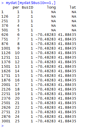
To see the problem with this data set, examine the data for the first business using the command mydat[mydat$BusID==1,]. Here's a screenshot of the output.



This problem occurs throughout the data set and we would like to just substitute the lat-long values we have for the right missing ones.

How did I solve my NA problem? I used aggregate(), a function that quickly and conveniently collapses a data frame by a factor or list of factors. With aggregate(), you can take the mean, compute the max, compute the min, sum the values or compute the standard deviation by the levels of the collapsing factor. The aggregate() function also has a na.rm option that allows us to easily ignore the NA values (useful here). In our example, we could collapse by taking the mean or computing the max or the min; the result will be the same because latitude and longitude do not vary for the same business over time.

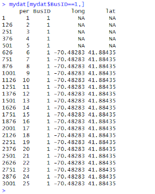
Let's collapse by taking the mean withing each level of BusID. The result of my use of aggregate() is a data frame that upon merging with the original data frame (using merge()), fills in the missing latitude and longitude values. The following code implements this strategy to fill in the NAs in our simulated data set.



Before leaving you to have fun with aggregate() and merge(), several points are worth mentioning.

First, the aggregate() function requires that the collapsing factor(s) is (are) stored in a list. This is why the code uses list(BusID=mydat$BusID) when mydat$BusID would seem more natural. The list() part is necessary to get aggregate() to work.

Second, it is useful for merging in the second step to give the attribute in the list the same name as the variable name in the original data frame. The BusID= part of the list(BusID=mydat$BusID) command is a convenient way to prepare the resulting data frame for merging.

Third, my code uses -c(3,4) to drop the 3rd and 4th columns of the original data frame (the ones with the original lat-long data) before merging it with the collapsed latlong data frame. This is important so that the merge() command doesn't get confused about which columns to use for matching. If you leave these columns in mydat, R's merge will try to match the values in those columns as well (because they have a common name with those columns in latlong).

Finally, the data in this example are in a different order now that we merged on BusID. If this bothers you, you can use order to sort the data set by time period as in

myfinaldat=mycleandat[order(mycleandat$per),]

As this last step is purely a cosmetic change to the data set that will not affect subsequent analyses, you can leave it out.

Although this example was my solution to a rather specific problem, it illustrates how to use some useful commands. To the extent that these commands are widely applicable to other problems, I hope you find uses for these commands in related applications.

Recreational R: Simulating a Card Trick

In this post, I simulate an interesting card trick, which was described by a friend of mine named Xan. Here's Xan's description of the card trick:

• I put a deck of cards down face up on the table. Meanwhile you think of a secret number between 1 and 10 -- for exposition let's say you pick 4.
• One by one, I discard cards from the top of the deck. When we get to the 4th card -- and let's call it your special card -- you look at the number. For exposition, let's say your special card happens to be a 7. Then 7 secretly becomes your new number. Note that I don't know your special card.
• I keep flipping cards, and 7 cards later, you have a new special card and number yet again. Note that I still don't know your special card.
• This process continues -- me flipping cards at a constant rate, you secretly updating your special card and counting up to the next one -- until I decide to stop.

But I don't just stop on any card. I stop on your current special card. Which I'm not supposed to know.

The following script file is a crude first approximation to simulating this card trick for the first 150 cards. This crude strategy is simple: (1) Simulate a sequence of 150 cards, (2) Pick a starting value -- might as well do all of them at once, and (3) Implement Xan's trick on all of them (that's what the for loop does).



Here's the result of running this script three times and plotting 10 secretnum sequences: one for each starting value. Each run starts with 10 distinct secret numbers (with a default chance of 0.1 of the trick "working"), and in my three runs, every starting value of the secret number eventually converges on the same sequence of secret numbers. More on the intuition for this here.



There are a couple of things wrong with this simulation that may have stacked the deck in favor of it working. I fixed these before writing this post, but I think it is useful to see the quick and dirty solution before adding frills and realism (which is what I do now).

1. I merely simulated my 150 cards using a uniform distribution on 1 to 13 (then forcing the face cards 11, 12 and 13 to be 10s). This is equivalent to sampling with replacement, which may have different properties than sampling without replacement.
2. There are only 52 cards in a deck. How would this work with only one shuffle, but passing through the deck (almost) three times until 150 cards? This is a different problem. Maybe you wouldn't expect much improvement after one pass through the deck (because you've seen that sequence of cards before).

A clever use of the rep() command can create a "fresh" deck of cards without suit distinction (which doesn't matter for the trick). Now, how to use R to shuffle a deck of cards? The sample() command, of course. With this technique in mind, I wrote the following function to compute the probability that the trick works (that is, the probability that two independent guesses end up at the same secret number) given a number of decks and a number of passes through the entire stack of cards (for a given shuffle).



Once you define this function, we can save the probability of the trick working for 1000 different shuffles of the cards. This script does it for one deck and one pass through the deck.



Then, we can take the average probability, which feels like the probability the trick works (unconditional on the particular shuffle or guess of a secret number). In the simulations I have run, this number turns out to be around 0.74 for one deck and one pass through the deck and about 0.86 using one deck and passing through twice. There's not much improvement after the second pass through of the deck.

In case you're interested, here are the results for up to 3 decks and up to 5 passes through the set of cards. It is always better to have more decks, but two passes through two decks is about enough to virtually guarantee that the trick works.



Update: In case you are wondering, I also coded it up with a 0.01 probability of forgetting to update on any given flip of the card. Here's the table of results in this case.



It's no surprise: For forgetful people, the trick is less successful and there isn't much point in reaching for a second deck.

An Application of boot() to IV regression

Bootstrapping standard errors can be a useful technique when obtaining closed form for the standard error formula is difficult or intractable. In this post, I give an example of how to use R to create a bootstrap sampling distribution in the context of IV regression. Specifically, I use boot() to automatically augment a function of mine to resample the indices of my data set with replacement (see the code in the function below).

In my application, I present a function that uses the boot library to report bootstrap standard errors for an instrumental variables regression. My ivboot() function builds on the iv() command I wrote for the tonymisc library.*

Now, onto the ivboot() example. Start by loading the tonymisc library and some data from the library, as well as the boot library.



We can run the following R script to define the function ivboot().



When applied to data and an IV regression model, the ivboot() function creates an IV regression object that -- when tonymisc is loaded -- is compatible with mtable() output. The only difference between an ivboot()-created object and an iv() object is that the ivboot() object has standard errors that are based on the bootstrap distribution of the coefficient estimates (Statistics other than the second-stage coefficient estimates are not bootstrapped).

Here is some code to compare the bootstrap output to the analytical standard error output:



On this small sample (N=100) of simulated data, the ivboot() command took less than a minute to run on my computer (timing of may vary depending on your computer). For much larger data sets, this will be slower. If you have a larger problem or lower standards (or higher standards, your choice), you can use the boots option to ivboot() to specify the number of bootstrap samples. Currently, I have set the default to 500, but you could specify boots = 200 if you want the command to run faster (boots = 10 will make it run even faster, but I don't recommend that!).

Here is the mtable() output, which can easily be ported into LaTeX using the toLatex() command.


*This standard output from an mtable() extension to my iv() command provides quite a bit of information in a convenient format. Another nice feature of iv() is that iv()-created objects have first-stage summary information readily stored in the object for extraction and analysis.